How to Create a Drop Down List in Microsoft Excel

Are you looking to create a dropdown list in Microsoft Excel? If so, then you’re in the right place. Microsoft Excel is a great tool for creating a professional schedule, data structures, or a record. Like other convenient tools, the drop-down list is one of the useful tools that allows individual users to simplify input data.

By adding the input data to the drop-down list, you can quickly select the data. This will save the users time, prevent spelling mistakes in a cell, and make data input much faster. Here, we’ll share with you two different ways to make a drop-down list in an Excel worksheet.

Ways to Create a Drop-Down List in Excel Worksheet

The Excel drop-down menu is mainly used for entering data from predefined items in a spreadsheet. By selecting the cell data, you will see a little arrow next to the selected cell. You can click on it to select the input data you’d like to add to the cell.

1. Make a Drop Down List in Excel From a Range of Cells

Excel comes with a “Data Validation” tool that allows the users to create a drop-down menu by using it. In addition, there is a benefit of creating a drop-down dynamic, which means you can change the cell data at any time.

Here’s how to make a drop-down menu in Excel from a range of cells:

1. Open the Microsoft Excel worksheet and navigate where you would like to add the list.
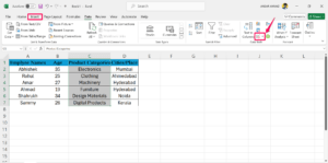
2. Select the range of cells that you want to add to the drop-down menu.
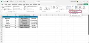
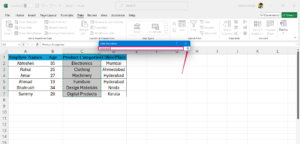
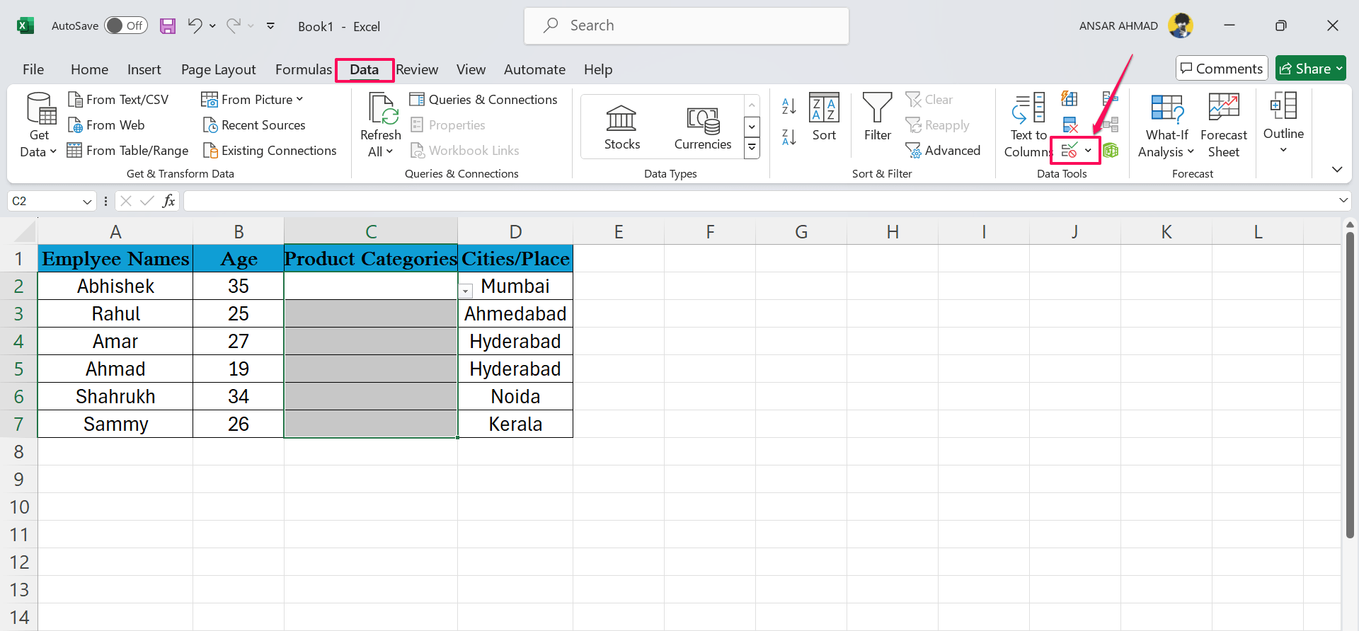
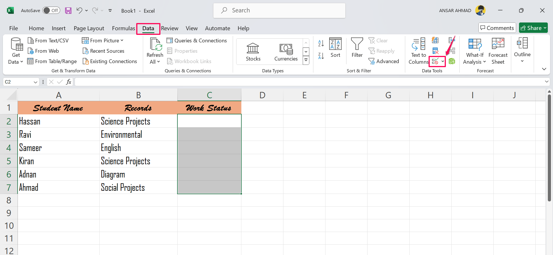
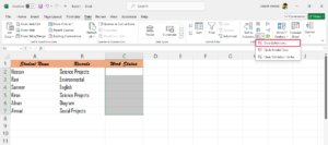
3. Click on the Data tab located at the top bar. Then, click on the Data Validation icon drop-down menu.
   
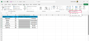
4. Now, choose the “Data Validation” option from the pop-up menu.
   
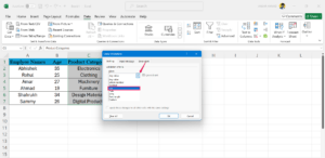
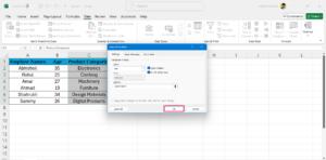
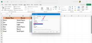
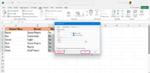
5. Click the Allow drop-down menu in the Data Validation dialog box and select List.
   
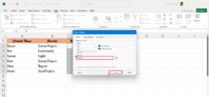
6. In the Source section, click the “Up” arrow located on the right side to add the cell range. This will open another window.
   
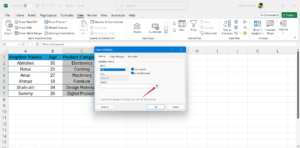
7. Here, select the cell range for which you want to create a drop-down list. You can click and drag the cursor to select the cell range.
8. After selecting the cell range, click the “Down” arrow towards the right side of the dialog box.
   
9. Once you added the cell range to the Source, click the “OK” button to confirm changes.
   

Now you will see the drop-down arrow next to the cell range you have selected. Simply click the down arrow and it will show you a list. Now, select the data and it’ll be added to your cell.

2. Make a Drop Down List in Excel with a Yes/No Option

You can also create a drop-down list in the Excel worksheet according to your defined names as list items. For instance, here we are taking the Yes/No option for your reference. You can define the name according to your needs.

1. Open the Excel worksheet.
2. Select the cells where you want to make the drop-down list.
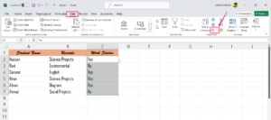
3. Click on the Data tab located at the top ribbon. Then, click on the Data Validation drop-down menu in the “Data Tools”.
   
   
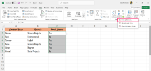
4. Now, choose the “Data Validation” option from the pop-up menu.
   
5. Under the Validation criteria, click on the drop-down arrow for the Allow option and select “List.”
   
   
6. Click on the “Source” text box and type the drop-down option you want to add.
7. Type the list of options by using the commas and ensure it is separate. For instance, we are typing “Yes” and “No.” You can write them as “Yes,No.”
8. As soon as you add the options, click the “OK” button to confirm the changes.
   

Now you will see a small arrow icon with the drop-down menu on your selected cell’s right side. By clicking on the arrow, you will see your input options (Yes, No). Click on it and it will be added to your cell.

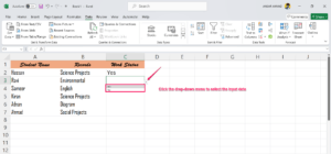
Note: We have shown you a Yes or No option for your reference. You can define names as list items accordingly.

How to Show Error Message for Invalid Data in Drop-Down Section

Drop-down menus allow users to select the value data they wish to add. But you can still change the data by inserting it into your cell. To avoid the unwanted value to the cell, you can show an error message if invalid data is added.

1. Open the worksheet in Excel and select the cells to add the error alert.
2. Click on the “Data” at the top ribbon. Then, click on the Data Validation drop-down menu in the “Data Tools”.
   
   
   
3. Select the Data Validation option from the pop-up menu.
   
   
4. If you have not specified the drop-down menu, ensure to specify the one in the Settings tab.
   
5. Under the Data Validation, click on the “Error Alert” tab.
6. Then, checkmark the “Show error alert after invalid data is entered” option.
   
7. Click the Style drop-down menu and select “Stop, Warning, and Information.”
8. After selecting the Style type, select the Title and type “Invalid Data.”
9. Then, click on the “Error message” content and input “The data you entered is invalid.”
   
   10. Once you add the data, click on the “OK” button to confirm changes.

How to Remove Drop-Down List in Excel

Now you know how to create a drop-down menu in Excel from a range of cells. If you don’t want to insert a drop-down menu and want to remove it, here’s how to do it.

1. Open the Excel worksheet.
2. With the cells selected, click on the “Data” tab in the top ribbon and click the Data Validation drop-down arrow icon in the “Data Tools.”
   
3. Then, select “Data Validation” from the pop-up menu.
   
4. Under the Data Validation dialog box, choose the “Settings” tab and click the “Clear All” button.
5. Finally, click the “OK” button to save changes.
   

Bottom Line

That’s it. This is how you can easily create a dropdown list in Microsoft Excel. We’ve listed two different ways to create a drop-down list that will help you improve your Excel data efficiency.

If you've any thoughts on How to Create a Drop Down List in Microsoft Excel, then feel free to drop in below comment box. Also, please subscribe to our DigitBin YouTube channel for videos tutorials. Cheers!